Evaluation

Once we have constructed an algorithm and plotted equity on historical data, we need to use a set of criteria to evaluate the performance. All current competition rules are available here.

Statistics

First, to estimate the profitability of the algorithm, we measure the Sharpe ratio (SR), the most important and popular metric. For our platform, we use the annualized SR and assume that there are ≈252 trading days on average per year. Annualized SR must be at least greater than 1 for the In-Sample test. «calc_stat» function allows to calculate of all the statistics of an algorithm.

Function

qnt.stats.calc_stat(data, portfolio_history, slippage_factor=0.05, roll_slippage_factor=0.02,
              min_periods=1, max_periods=None,
              per_asset=False, points_per_year=None)

Parameters

Parameter	Explanation
data	xarray DataArray with market data of the companies your algorithm invests in.
portfolio_history	xarray DataArray filled with portfolio weights, corresponding to the investing algorithm.
slippage_factor	Transactions are punished with slippage equal to a given fraction of ATR14. We evaluate submissions using 5% of ATR14 for slippage. Read more about slippage here
roll_slippage_factor
min_periods	minimal number of days
max_periods	max number of days for rolling
per_asset	calculate stats per asset
points_per_year

Output

The output is xarray with all statistics.

Output columns
equity
relative_return
volatility
underwater
max_drawdown
sharpe_ratio
mean_return
bias
instruments
avg_turnover
avg_holding_time

Example

Assume you chose «buy and hold» strategy and formed output weights:

import qnt.data    as qndata
import datetime as dt
import qnt.stats as qnstats        # key statistics
import qnt.graph as qngraph        # graphical tools
from IPython.display import display
# load historical data
data = qndata.load_data(
                       tail = dt.timedelta(days=4*365),
                       dims = ("time", "field", "asset"),
                       forward_order=True)
is_liquid = data.loc[:,"is_liquid",:].to_pandas()
# set and normalize weights:
weights = is_liquid.div(is_liquid.abs().sum(axis=1, skipna=True), axis=0)
weights = weights.fillna(0.0)
#convert to xarray before statistics calculation
output = weights.unstack().to_xarray()

When the weights are formed, one can calculate statistic in order to evaluate algorithm on a historical data:

stat = qnstats.calc_stat(data, output, slippage_factor=0.05)
display(stat.to_pandas().tail())

field time	equity	relative_return	volatility	underwater	max_drawdown	sharpe_ratio	mean_return	bias	instruments	avg_turnover	avg_holding_time
2020-09-01	1.547375	0.007302	0.213420	0.000000	-0.382386	0.549581	0.117291	1.0	967.0	0.026296	83.810199
2020-09-02	1.565288	0.011577	0.213385	0.000000	-0.382386	0.564401	0.120434	1.0	967.0	0.026506	85.397114
2020-09-03	1.514099	-0.032703	0.213932	-0.032703	-0.382386	0.518395	0.110901	1.0	967.0	0.026526	85.397114
2020-09-04	1.501310	-0.008446	0.213872	-0.040873	-0.382386	0.506844	0.108400	1.0	967.0	0.026522	85.397114
2020-09-08	1.472630	-0.019104	0.213991	-0.059196	-0.382386	0.480810	0.102889	1.0	967.0	0.026517	165.190915

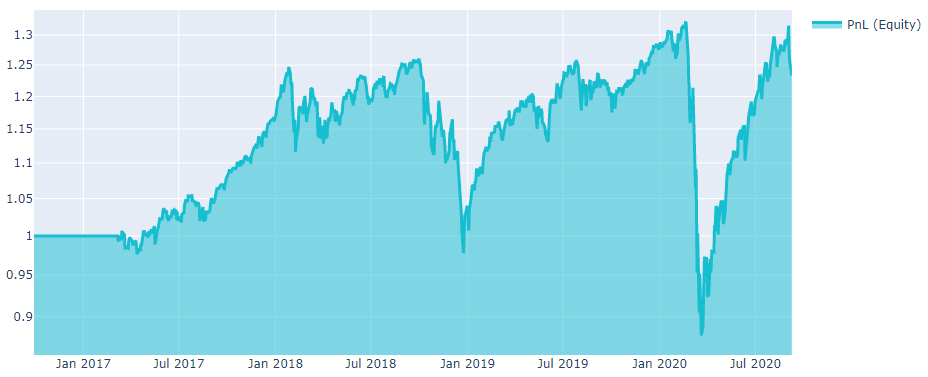
# show plot with profit and losses:
performance = stat.to_pandas()["equity"]
qngraph.make_plot_filled(performance.index, performance, name="PnL (Equity)", type="log")

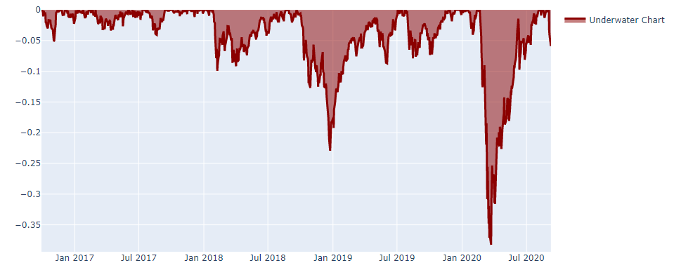
# show underwater chart:
UWchart = stat.to_pandas()["underwater"]
qngraph.make_plot_filled(UWchart.index, UWchart, color="darkred", name="Underwater Chart", range_max=0)

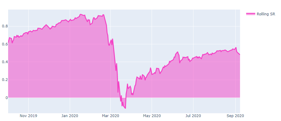
# show rolling Sharpe ratio on a 3-year basis:
SRchart = stat.to_pandas()["sharpe_ratio"].iloc[(252*3):]
qngraph.make_plot_filled(SRchart.index, SRchart, color="#F442C5", name="Rolling SR")

Exposure filter

It is worth using a few instruments for the trading algorithm. Even if the strategy is right, unpredictable world events/news may cause irreparable damage (for instance, 1 and 2).

A good way to diversify risks is to increase the number of instruments in the investment portfolio. The algorithm can be submitted only when it meets the following criterion - the maximum investment in each instrument does not exceed 5 percent of the invested capital.

However, this rule contains concessions aimed at eliminating disputable situations. Below is a more detailed description of the requirement. Let“s introduce MP - the maximum percent of the invested capital, distributed per instrument. The exposure filter is passed if one of the conditions is met:

• The MP can be from 5% to 10% no more than 5 days per year.

• The cumulative excess of the MP for all shares is calculated. The average daily value should not exceed 2 %.

The hard limit is 10%. It means that if MP exceeds 10% your algorithm does not pass the filter.

One can use the check_exposure function in order to check this requirement.

Function

check_exposure(portfolio_history,
                   soft_limit=0.05, hard_limit=0.1,
                   days_tolerance=0.02, excess_tolerance=0.02,
                   avg_period=252, check_period=252 * 3)

Parameters

Parameter	Explanation
portfolio_history	output xarray DataArray
soft_limit	soft limit for exposure
hard_limit	hard limit for exposure
days_tolerance	the number of days when exposure may be in range from 0.05 to 0.1
excess_tolerance	max allowed average excess
avg_period	period for the ratio calculation
check_period	period for checking

Output

The output is bool. True indicates successful passing the filter.