What is Algorithmic Trading?

«Algorithmic trading is a process for executing orders utilizing automated and pre-programmed trading instructions to account for variables such as price, timing and volume. An algorithm is a set of directions for solving a problem. Computer algorithms send small portions of the full order to the market over time.» - Investopedia.

Вasic concepts

Algorithmic trading means that the decision to buy or sell financial securities on the stock exchange is made based on a predetermined algorithm, with the intent to make a profit. On our platform, it is a python script that takes historical data as an input and gives a decision to buy/sell stock as output.

Say we have a capital $1M and want to invest in a portfolio consisting of three stocks: Apple Inc (AAPL), Alphabet Inc Class C (GOOG), Tesla Inc (TSLA). Let“s have a look at the open price of these stocks for some period. Open is the price at which a security first trades upon the opening of an exchange on a trading day. We use historical data from the NASDAQ exchange as input:

date	AAPL	GOOG	TSLA
Mar 02, 2020	282.28	1,351.61	711.26
Mar 03, 2020	303.67	1,399.42	805.00
Mar 04, 2020	296.44	1,359.23	763.96

Table 1: Stock open price in USD. NASDAQ exchange.

Now we need to come up with an algorithm by which our capital will be allocated between stocks. The algorithm is an intelligent search of some world event reflected in data. Usually, it is based on some idea. Suppose we have a hypothesis - invest more if open price is low. A hypothesis can be expressed through the formula:

\[\label{alpha1} \frac{1}{\textbf{open}},\]

Hereinafter we will stand bold symbols for vectors. We can receive a matrix form of the algorithm by applying formula (2) to the table 1:

date	AAPL	GOOG	TSLA
Mar 02, 2020	0.00354258183	0.00073985839	0.00140595562
Mar 03, 2020	0.00329304837	0.00071458175	0.00124223602
Mar 04, 2020	0.00337336391	0.00073571065	0.00130896905

Table 2: Matrix form of the algorithm.

Capital is distributed in proportion to the values of the matrix. To receive the shares of capital invested in each stock, the matrix (table 2) must be normalized \(` l_1 `\)) norm) to one for each day:

date	AAPL	GOOG	TSLA
Mar 02, 2020	0.6228	0.1301	0.2472
Mar 03, 2020	0.6273	0.1361	0.2366
Mar 04, 2020	0.6226	0.1358	0.2416

Table 3: Final weights of the algorithm.

Thus, $1M·0.6228 = $622,800 was allocated for AAPL on Mar 02, 2020; GOOG and TSLA received $130,100 and $247,200 correspondingly. Matrix values (3) are called weights of the algorithm.

Long Position vs. Short Position

---

To sell a stock, one just needs to assign it a negative weight in the algorithm.Assume, you have the following weights:

date	AAPL	GOOG	TSLA
Mar 02, 2020	0.4	0.4	-0.2

The positive sign means that we hold a long position (buy shares); the negative sign means we hold a short position (sell shares). Thus, the capital 1M will be allocated in the following proportions: $400,000 to AAPL; $400,000 to GOOG; $-200,000 to TSLA.

Details

For our platform, we use a simplified treatment of short positions and mirror long positions. For a real-environment trading one needs to remember that short positions are associated with higher risks. An investor selling shares that he does not yet own (as a rule, from his broker“s account) is obligated to buy them back after a while. Thus, the investor expects a fall in prices and plays against the market. It leads to several risks:

• Some stocks are hard to borrow. The reason is high demand, a limited number of securities and so on. For a short position for such securities, the broker charges an additional fee.

• The short seller is responsible for paying dividends on shares to the person from whom they were borrowed.

• The potential losses in a short sale can be endless, because theoretically the maximum price of shares is unlimited. On the other hand, the share price will not fall below zero, so the maximum profit is limited.

• Even if the estimate is correct, the moment may be inappropriate. It is extremely unprofitable to hold a short position at a rising price for a long time.

Relative returns

The investment portfolio is redistributed according to the algorithm once a day (the exchange has 252 working days a year). Redistribution occurs at the beginning of the day. For our platform, we assume that the purchase of shares occurs at the open price.

Equity grows with the correct prediction of price changes. The daily change in equity is estimated after the end of the trading day and strongly depends on the close price. Close is the price at which a security last trades on a trading day.

Algorithm results, calculated on historical data, are usually presented on an equity graph in order to understand the behaviour of the cumulative profit. In our platform, we set initial equity to 1, so it can be scaled easily.

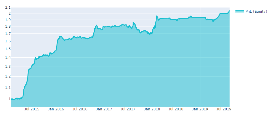Pic. 1

Relative returns simply indicate how much the capital has changed. For the \(`i^{th}`\) day we introduce the relative returns (rr) in unit fractions:

\[\label{equity1} \text{rr}[i] = \frac{\text{equity}[i]}{\text{equity}[i-1]} - 1,\]

Details

Sometimes it“s important to understand how equity (cumulative profit, PnL) is calculated. Say we allocate our capital in a proportion to the vector of weights for the \(`i^{th}`\) day. Thus we buy shares at open price and receive the following positions:

\[\label{position} \textbf{pos}[i] = \left( \textbf{weights}[i]\cdot\text{equity}[i] \right)/\textbf{open}[i],\]

where bold variables stand for vectors in the space of shares; division is elementwise. For the next day, an algorithm will generate a new vector of \(`\textit{weigths}[i+1]`\) that will redistribute our capital into new positions. Redistribution of portfolio instruments leads to capital losses associated mainly with the broker“s commission and the slippage.

It is quite clear that the greater part of the capital we must redistribute, the more broker“s commission affects our profit. For real trading, slippage has a more significant impact on profit than the commission, so in our platform, we only consider slippage.

What is the slippage? We need a buyer/seller to sell/buy any shares. If there is no offer on the exchange, the order is opened at a new price. Thus, we buy the desired number of shares in parts, using offers to buy/sell a specific number of shares at a specific price. We calculate slippage according to the following formula:

\[\label{slappage} \text{slippage}[i] = abs(\textbf{pos}[i] - \textbf{pos}[i-1])\cdot \textbf{ATR}(14) \cdot 0.05,\]

where \(` \textbf{ATR}(14) `\) - is a market volatility indicator. The Average True Range (\(` \textbf{ATR}(N) `\)) indicator is a moving average (MA) over N days of the true range (TR) values:

\[\begin{gathered} \label{ATR} \textbf{TR}[i] = max( \textbf{high}[i] - \textbf{low}[i]; \textbf{high}[i] - \textbf{close}[i-1]; \textbf{close}[i-1] - \textbf{low}[i]), \end{gathered}\]

\[\label{ATR2} \textbf{ATR}(N) = MA(\textbf{TR},N).\]

Now we can introduce the equity formula for the i day:

\[\begin{split}\begin{gathered} \text{equity}[i] = \text{equity}[i - 1] + (\textbf{open}[i] - \textbf{close}[i-1]) \cdot \\ \textbf{pos}[i-1] + (\textbf{close}[i] - \textbf{open}[i]) \cdot \textbf{pos}[i] - \text{slippage}[i] \label{equity}\end{gathered}\end{split}\]

Algorithm quality

---

Once we have constructed an algorithm and plotted an equity on a historical data, we need to use a set of criteria to evaluate the performance. All current competition rules are available here.

Sharpe Ratio

First, to estimate the profitability of the algorithm, we measure the Sharpe ratio (SR), the most important and popular metric. For our platform, we use the annualized SR and assume that there is ≈252 trading days on average per year. The annual SR formula for N days is presented below:

\[\label{SR_final_first} \text{SR} = \frac{\sqrt[N]{[\prod\limits_{i=1}^{N} (rr_i + 1)]^{252}} - 1}{\sqrt{\frac{252}{N}\sum\limits_{i=1}^{N} (rr_{i} - \overline{rr}) }},\]

where \(` rr_i `\) stands for the daily relative returns (of the i“th day), \(`\overline{rr}`\) denotes the expected value.

The numerator is an average daily return. The book size changes with the size of equity, thus the numerator is a geometric mean.

The denominator is a standard deviation of the portfolio’s excess return. Another way to think about the denominator is that it means volatility.

Thus, the Sharpe ratio is the return per unit of risk (volatility). The greater the Sharpe ratio, the better (Fig.2). To submit a strategy successfully, the SR should be higher than 1 over the last 3 years.

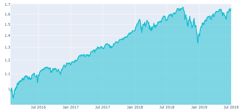
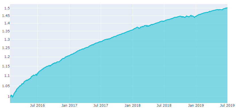Figure 2: Equity charts for different algorithms. Upper: \(` \text{SR} = 1.28 `\). Lower: \(` \text{SR} = 7.62 `\)

Details

In 1994, William Sharpe defined the Sharpe ratio as:

\[\label{SR_1} \text{SR} = \frac{E(R_p - R_f)}{\sigma_p},\]

where \(` R_p `\) - return of the portfolio , \(` R_f `\) - risk-free rate, \(` E(R_p - R_f) `\) - s the expected value of the excess of the portfolio return over the benchmark return, \(` \sigma_p `\) - standard deviation of the portfolio“s excess return. We assume risk-free rate to be zero (alternative way to compute the Sharpe ratio is to set S&P 500 total return as a risk-free rate). For N trading days:

\[ \label{SR_2} \text{SR} = \frac{\text{average daily return}}{\text{daily volatility}} = \frac{\sqrt[N]{\prod\limits_{i=1}^{N} (rr_i + 1)} - 1}{\sqrt{\frac{1}{N}\sum\limits_{i=1}^{N} (rr_{i} - \overline{rr}) }},\]

where \(` \overline{rr} `\) - denotes the expected value of relative returns. The book size changes with the size of equity, thus the numerator is a geometric mean. Now we introduce the SR, scaled on an arbitrary period \(` T `\):

\[\label{SR_final} \text{SR} = \frac{\sqrt[N]{[\prod\limits_{i=1}^{N} (rr_i + 1)]^T} - 1}{\sqrt{\frac{T}{N}\sum\limits_{i=1}^{N} (rr_{i} - \overline{rr}) }}.\]

For annual Sharpe ratio one can put T= 252 - trading days per year. We use annual (T= 252) Sharpe ratio (11) to estimate algorithms on our platform.

Uniqueness

Every good trading algorithm is a signal that reflects the imperfection of the market. The more capital involved in the signal, the less marginal this signal. A good algorithm must minimize intersection with well-known and already existing signals. Uniqueness can be defined as a maximum correlation of the algorithm to the pool of the existing algorithms:

\[r_{XY} = \frac{\text{cov}_{\textbf{X}\textbf{Y}}}{\sigma_{\textbf{X}} \sigma_{\textbf{Y}}} = \frac{\sum (\textbf{X} - \overline{\textbf{X}})(\textbf{Y} - \overline{\textbf{Y}})}{\sqrt{\sum (\textbf{X} - \overline{\textbf{X}})^2(\textbf{Y} - \overline{\textbf{Y}})^2}}\]

where \(` \textbf{X}, \textbf{Y} `\) are daily relative returns. The lower the correlation, the better. According to the rules, your algorithm must have a correlation coefficient lower than 0.9 over the last 3 years; otherwise, you need to have the largest Sharpe ratio among the correlated algorithms.

Diversification of risks

It is worth to use a few instruments for the trading algorithm. Even if the strategy is right, unpredictable world events/news may cause irreparable damage (for instance, 1 and 2).

A good way to diversify risks is to increase the number of instruments in the investment portfolio. After that we can set a maximum stock weight to 0.05. It means that we will allocate no more than 5% of our equity to the each stock.

There are many such news every year - they merge with the information noise and we forget them. However, they are reflected in historical data and strongly affect profit in the future. According to the rules, your algorithm must pass exposure filter. You can use the suggested tools to avoid filtering out the algorithm due to exposure filter.

Is and Os

---

Overfitting is easy. If one tries a significant amount of algorithm configurations, backtest can be fitted to any desired performance. The number of guidelines can help to avoid overfitting and estimate a real algorithm value.

In sample

By «sample» we mean a data sample. Thus, in-sample (IS) is an observed historical data, an analogue of the training set in machine learning. In order to prevent overfitting, one can test the model using a longer history or improve in-sample requirements.

Out of sample

The out-of-sample (OS) is an analogue of the testing set in machine learning. It is real-time data. We take each algorithm, test it day by day in a real environment and monitor its performance. It is wrong when an algorithm changes its strategy with time. All conditions must be consistent.

Competition

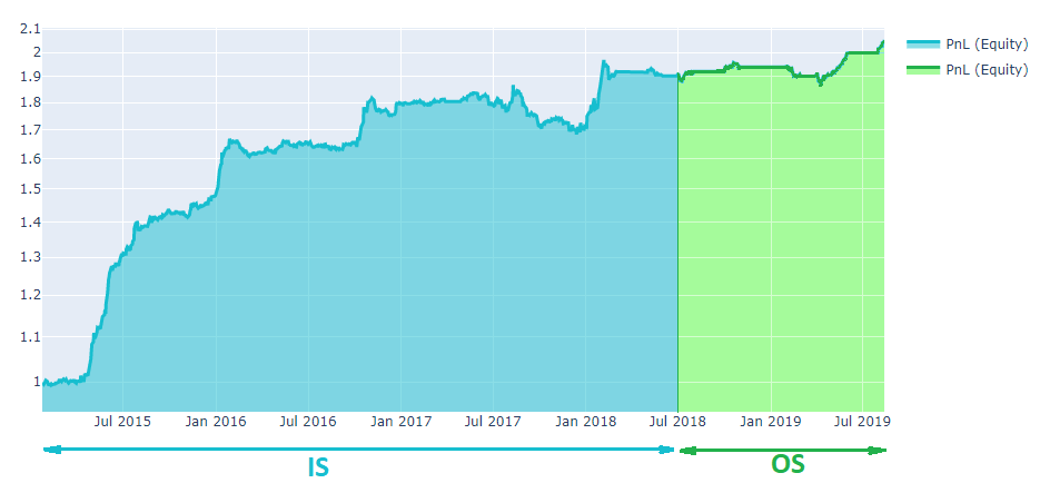
Say you are participating in QuantNet Contest in the 6 months competition and create an algorithm for stock trading. According to the rules, you have a good Sharpe (>1) and low correlation (<0.9) over the previous 3 years. The backtest for this 3 years is in-sample (Fig.3). Say we measure SR in-sample - SR_IS. The real time test for 6 months is out-of-sample and gives SR_OS. All strategies are rated by min(SR_IS, SR_OS). The larger the better.

Improving the algorithm

Neutralization

---

Let“s analyse the stock performance of 500 large companies listed on stock exchanges in the United States. The so called index S&P500. As one can see, the market growth on average. S&P500 return varies widely from a few percent to over 20% in some years. Does it mean that simply opening a long positions is a good idea?

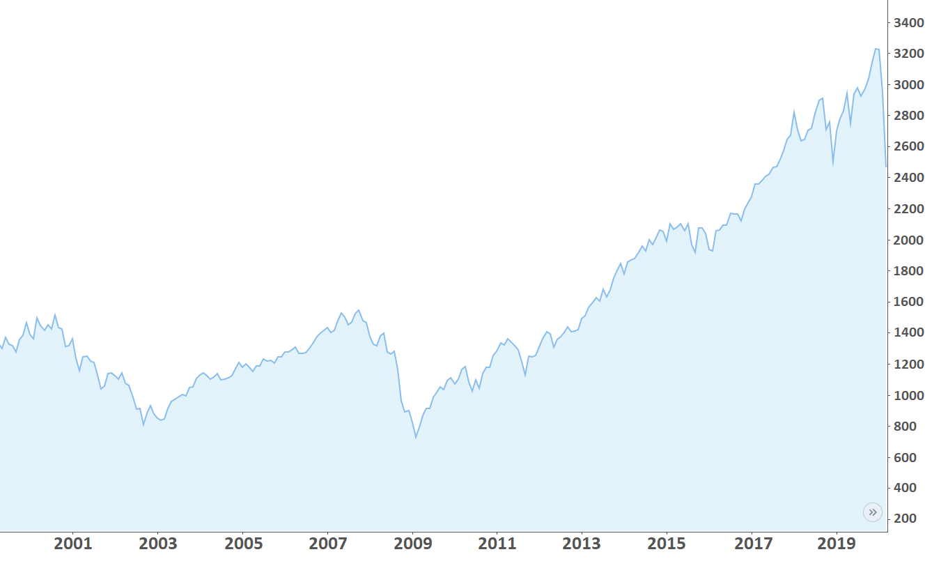
Despite the growth, the Sharpe ratio of S&P500 is less than 1. One of the main reason - periodic financial crises. There are some of them:

• 1987 year. «Black Monday.» The Dow Jones Index fell 22.6% in the United States. The reason is the massive outflow of investors from regional markets.

• 2000-2003. The Crash of the Dotcoms. The crisis caused by the massive investment of money in Internet projects.

• 2007–2008. Great Recession. The combination of banks unable to provide funds to businesses, and homeowners paying down debt rather than borrowing and spending, resulted in the Great Recession that began in the U.S. officially in December 2007 and lasted until June 2009, thus extending over 19 months.

The consequences of crises are visible on the chart and appear as market drops of up to 30%. It is dangerous to think that the crisis is horror stories from the past. The beginning of 2020 is marked by the fall of the economy caused by Coronavirus.

Neutralization

We can exclude the market influence by balancing long/short positions for our algorithm. So, it will be a market-neutral. The neutralization could be done for the whole market or each industry (or smaller group). Mathematically, market neutralization is elementary.

Say, we a have a vector of weights_i for i day, given by the algorithm. In order to make the algorithm a market-neutral, one needs to apply the following equation for each day:

neutralized_weights_i = weights_i - mean(weights_i).

Now the mean of weights for each day is zero. It means that we neither invest money nor withdraw it from the market.